
Common Formula Errors in Google Sheets and Fixes
Most Google Sheets formula errors come from just 5 issues: syntax mistakes, broken references, lookup misses, data-type mix-ups, and bad math.
If I need to fix a formula fast, I check things in this order:
- Syntax first: parse errors and
#ERROR! - References next:
#REF!and blocked array output - Lookups after that:
#N/A - Data and math last:
#VALUE!,#DIV/0!,#NAME?, and#NUM!
That order matters. In many cases, the problem is not the whole formula. It is one bad range, one misspelled function, or one number stored as text. Even a small issue can throw off fleet reports, AUE tracking, or bulk admin work.
Here’s the short version of what I’d keep in mind:
- Parse error = Sheets can’t read the formula
#ERROR!= the formula shape is fine, but the function call is wrong#REF!= the formula points to a deleted or blocked range#N/A= the lookup value was not found#VALUE!= text showed up where a number or date was expected#DIV/0!= something tried to divide by zero or blank#NAME?= function or named range is spelled wrong#NUM!= the input numbers or dates do not work for that formula
A good first move is to test the formula in parts. That makes it easier to spot whether the failure comes from the formula itself or from the source data.
| Error | What it usually means | First fix to try |
|---|---|---|
| Formula parse error | Bad syntax | Check commas, quotes, and parentheses |
#ERROR! |
Wrong function setup | Check spelling and argument order |
#REF! |
Broken reference | Restore or repoint the range |
#N/A |
Lookup miss | Check spaces, types, and lookup column |
#VALUE! |
Wrong data type | Convert text to number or date |
#DIV/0! |
Zero/blank divisor | Add an IF check |
#NAME? |
Misspelled name | Fix function or named range spelling |
#NUM! |
Invalid numeric input | Check dates, limits, or negative values |
The main idea is simple: fix structure first, then ranges, then data. That solves most Sheets formula problems without rewriting everything.
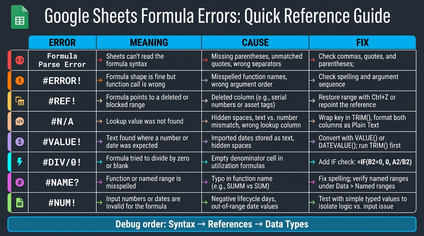
Google Sheets Formula Errors: Quick Reference Guide
Common Formula Errors in Google Sheets and How To Fix Them
sbb-itb-c68f633
Parse and Syntax Errors: Fix Formula Structure First
Parse errors are usually the first formula problems you'll run into. Google Sheets can't read the formula structure, so it stops right there before it even looks at your data. Start with structure. The quick comparison below helps you tell structure issues apart from logic issues.
| Error Type | Symptom | Likely Cause | Fastest Fix |
|---|---|---|---|
| Formula parse error | Formula won't evaluate | Missing parentheses, unmatched quotes, wrong separators, spaces inside function names, or stray characters copied from another source | Rebuild the formula structure; verify comma separators in en-US Sheets |
| #ERROR! | Formula parses, but the function call still fails | Misspelled function names, wrong argument order, or incorrect nesting | Check spelling, argument sequence, and nested structure |
Formula Parse Error
A parse error means Google Sheets can't read the formula syntax at all. The usual troublemakers are unmatched parentheses, unclosed quotation marks, stray characters copied from emails or documents, and spaces inside function names.
Use the color-coded parentheses in the formula bar to match each pair. For example, =IF(AND(A1>0, B1>0), "Pass", "Fail") works. Remove one closing parenthesis, and the whole thing falls apart.
Each text string needs a straight double quote " on both sides. If the formula still won't work, paste it into plain text and retype any characters that look off. Weird formatting from another app can sneak in and break things.
If the formula came from another locale, swap semicolons for commas in en-US Sheets.
If the structure looks right but Sheets still rejects the formula, move to #ERROR! and check the function logic.
#ERROR! from Invalid Syntax or Function Structure
#ERROR! shows up when the formula structure is fine, but the function logic, order, or nesting is off.
Check the function name, argument order, and nesting before changing anything else. For example, =VLOOKUP(A1,B:C,2,FALSE) is valid. =VLOKUP(A1,B:C,2,FALSE) fails because the function name is spelled wrong. If the formula points to another sheet, put quotes around sheet names with spaces, like 'Sheet Name'!A1:B10.
With deeply nested formulas, test the innermost function in its own cell first. Then add each outer layer one step at a time. That approach is often faster on IT reporting sheets that mix imported asset data or user metadata.
If the formula starts running but gives you the wrong result, the problem is usually in the references or lookup ranges.
Reference and Lookup Errors: Check Ranges, Keys, and Deleted Cells
If a formula parses but still fails, the next place to look is the data behind it. In IT tracking sheets, #REF! and #N/A show up all the time, but they point to different problems. Here’s the quick read:
| Error | Meaning | Common IT Cause | First Step |
|---|---|---|---|
| #REF! | Reference is invalid or broken | Deleted column of serial numbers or asset tags | Check for recently deleted source columns; use Ctrl+Z to undo if the deletion just happened |
| #N/A | Value not found | Mismatched serial number, trailing space in a username, text vs. number formatting mismatch | Verify the lookup key actually exists in the source range; check for hidden spaces |
| Array spill blocked | Array formula can't expand | A cell in the formula's output path has a manually entered value | Clear the blocking cell so the array can populate |
#REF! from Broken or Invalid References
#REF! means the formula points to something that no longer exists. Deleted columns break references. Cleared cells don’t. In IT sheets, this often happens when someone deletes a column with device serial numbers or asset tags that a formula depends on.
If the deletion just happened, hit Ctrl+Z on Windows or Cmd+Z on Mac right away. That’s the fastest fix. If the file has already been saved or undo history is gone, check the formula bar and look for the part replaced by #REF!. That marks the broken reference. Then update it so it points to the right range.
Array formulas can fail in a different way. If someone types into a cell that the array needs to fill, the array can’t expand and throws #REF!. Hover over the error cell. Google Sheets will often show which cell is in the way. Remove that manual entry, and the array should fill as expected.
It also helps to use named ranges like AssetList instead of hard-coded ranges like A2:A500. And when you copy formulas, lock ranges with absolute references such as $A$2:$B$500.
#N/A from Lookup Mismatches
#N/A means the lookup itself worked, but it couldn’t find the value you gave it. In IT data, the usual culprits are hidden spaces, mixed data types, or a lookup range that starts in the wrong place.
A simple fix is to wrap the lookup key in TRIM() so leading and trailing spaces get stripped out before the search runs. If the same ID shows up as text in one place and as a number in another, format both columns as Plain Text. That small mismatch is enough to break a lookup.
Also check the lookup range itself. The search key has to be in the first column of that range. If your range starts one column too far to the right, every lookup can return #N/A even when the value is sitting there in plain sight.
Sheets-Based Admin Workflows Using Imported Metadata
When references break or lookup keys don’t match, admin tasks can fall apart fast. In AdminRemix workflows like Chromebook Getter and User Getter, imported IDs, OU moves, and AUE reporting fail when references break or lookup keys do not match.
Keeping source ranges in place, using TRIM() on imported IDs, and staying out of array spill ranges with manual entries prevents most of these issues.
Calculation and Data-Type Errors: Validate Numbers, Text, and Function Names
Once your references are stable, the next step is checking the values and calculations behind them. These errors usually mean Google Sheets got the wrong kind of input.
This table helps split value issues from calculation issues.
| Error | Most Likely Cause | Fastest Correction |
|---|---|---|
| #VALUE! | Text instead of numbers | Convert with VALUE() or DATEVALUE() |
| #DIV/0! | Zero or blank denominator | Guard with IF |
| #NAME? | Misspelled function or named range | Fix spelling |
| #NUM! | Invalid numeric input | Check date order |
#VALUE! and #DIV/0!
#VALUE! usually means the formula ran into text where it expected a number. Imported AUE dates or Support End Date fields often come in as text or placeholder values instead of numbers or dates. A quick way to check is with ISNUMBER(). If it returns FALSE, convert the cell with VALUE() or DATEVALUE().
Hidden spaces can also trip things up. That’s why it helps to run TRIM() first before trying the conversion.
#DIV/0! shows up when the denominator is zero or blank. You’ll see this a lot in utilization or cost-per-device formulas when a device count cell hasn’t been filled in yet. Use =IF(B2=0, 0, A2/B2) to handle zero on purpose instead of letting the formula fail.
If the math looks fine but Sheets still throws an error, shift your attention to function names and input limits.
#NAME? and #NUM!
#NAME? is usually a spelling mistake. For example, =SUMM(A2:A10) instead of =SUM(A2:A10) will trigger it right away. The same thing happens when a named range is missing or spelled wrong. Check Data > Named ranges and make sure the name matches exactly. This often pops up after copying formulas into a new sheet.
#NUM! appears when the formula structure is okay, but the numbers themselves aren’t. A date formula that produces negative lifecycle days is a common example. If you see #NUM!, try the same formula with a few simple typed values. That’s a fast way to figure out whether the issue is in the logic or in the input data.
Prevent Errors and Debug Complex Formulas More Efficiently
After you fix the error, a few habits can help keep complex IT formulas stable as source data changes.
Use IFERROR Only After Fixing the Root Cause
Once the formula works, add error handling only for edge cases you expect.
Use IFERROR for optional lookups, like asset owner fields. For example, =IFERROR(VLOOKUP(A2, UserTable, 3, FALSE), "Unassigned") returns Unassigned when a value is missing.
Don’t use IFERROR to cover up broken references or wrong ranges. If you wrap a broken formula, the error disappears from view, but the problem is still there. That can lead to bad asset counts or compliance metrics that look valid.
A cleaner option is IFNA for lookups where missing values are normal, and IFERROR for broader edge cases. First, test the formula without the wrapper. Then add IFERROR only where you know an edge case can happen.
A Simple Debugging Workflow for Large Formulas
If the error is still there after the basic fix, split the formula into smaller parts.
- Confirm the error starts here, not upstream.
- Check the inputs feeding the formula for blanks or type mismatches.
- Test each function on its own.
- Rebuild the formula one layer at a time.
- Compare it with the last working version in File → Version history.
For IT teams running large Sheets-based inventories and user data, modular formulas are worth the effort over time. Clean, consistent imports give those formulas a steadier base.
That workflow stops most repeat failures in changing IT sheets.
Conclusion: The Checks That Solve Most Sheets Formula Errors
The fastest path is still syntax first, then references, then data types. Standardize asset IDs, device statuses, and user fields to cut down on formula edge cases.
FAQs
Why does my Google Sheets formula work in one file but fail in another?
Usually, the problem isn’t the formula. It’s the data.
Hidden characters like line breaks, tabs, or non-breaking spaces can make two values look identical while acting like they don’t match at all. That’s why a lookup or match can fail even when everything seems fine at first glance.
Use CLEAN to strip out non-printable characters and TRIM to remove extra spaces. It also helps to check that the data types match across files. If one file stores a value as a number and another stores it as text, the formula can break even though the values look the same.
How can I tell if a lookup error is caused by hidden spaces or data type mismatches?
Use LEN to compare the character count before and after applying TRIM or CLEAN. If the counts don’t match, hidden characters or extra spaces are likely behind the lookup error.
Invisible characters - like leading or trailing spaces, line breaks, or non-breaking spaces - can make two values look identical on screen while still causing VLOOKUP or XLOOKUP to fail.
When should I use IFERROR instead of fixing the formula itself?
Use IFERROR when your formula is fine, but an expected error might pop up. A common case is dividing by zero or looking up a value that isn't there yet. It keeps those known errors from cluttering your sheet.
Don't use it to cover up basic issues like syntax mistakes or faulty logic. That just buries the problem and makes it harder to spot and fix.