10 Google Sheets Text Functions for IT Data Cleaning

Dirty data can derail your IT processes. From invisible spaces that break formulas to inconsistent capitalization that ruins pivot tables, messy data creates headaches. Google Sheets offers 10 text functions that simplify data cleaning, keeping your spreadsheets accurate and functional.

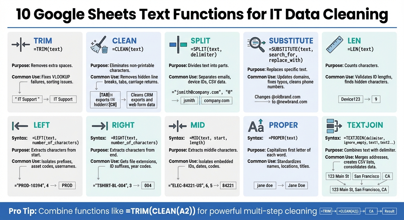
Key Functions:

• TRIM: Removes extra spaces.
• CLEAN: Eliminates non-printable characters.
• SPLIT: Divides text into parts based on a delimiter.
• SUBSTITUTE: Replaces specific text within a string.
• LEN: Counts characters in a string.
• LEFT: Extracts characters from the start of text.
• RIGHT: Extracts characters from the end of text.
• MID: Isolates characters from the middle of text.
• PROPER: Standardizes capitalization.
• TEXTJOIN: Combines text from multiple cells with a delimiter.

These tools help IT professionals fix common issues like mismatched data, hidden characters, and inconsistent formatting. Combining functions (e.g., =TRIM(CLEAN(A2))) can tackle multiple problems in one step. Whether you're cleaning metadata, processing logs, or managing IT assets, these functions streamline your workflow and improve data reliability.

1. TRIM

Function Purpose

The TRIM function is designed to tidy up text by removing extra spaces - whether they’re at the beginning, end, or even excessive spaces between words. Its syntax is straightforward: =TRIM(text). For example, if you use =TRIM(" IT Support "), it will return "IT Support", neatly eliminating unnecessary whitespace. This makes TRIM a go-to tool for cleaning up messy text data.

Use Case in IT Data Cleaning

In IT, spacing issues can cause all sorts of headaches. For instance, a simple trailing space can make VLOOKUP or XLOOKUP fail to match "User123" with "User123 ". Similarly, functions like COUNTIF and SUMIF might treat "Asset_01" and "Asset_01 " as completely different items, leading to inaccurate counts or mismatched inventory data. TRIM also fixes sorting problems caused by leading spaces. Without cleaning, entries like " Apple" could appear out of order, breaking dropdown lists or lookup rules.

Key Benefits

TRIM is especially powerful when working with large datasets. By combining it with ARRAYFORMULA, such as =ARRAYFORMULA(TRIM(A2:A)), you can quickly clean thousands of rows without manually applying the formula to each cell. It also pairs well with other functions like CLEAN. For example, =TRIM(CLEAN(A2)) not only removes extra spaces but also gets rid of non-printable characters. After splitting text with the SPLIT function, TRIM can tidy up any extra spaces that might show up in the resulting columns.

Despite its usefulness, TRIM does have some limitations.

Limitations

TRIM doesn’t handle non-breaking spaces (HTML character 160). To address this, you’ll need a workaround like =TRIM(SUBSTITUTE(A2, CHAR(160), " ")). It also doesn’t deal with tabs or line breaks, which means you’ll need the CLEAN function for those issues. Another thing to watch out for: when TRIM is applied to numbers, it converts them into text, potentially interfering with calculations. To avoid this, use "Paste Special > Values Only" after cleaning to replace the original data with the cleaned version.

sbb-itb-c68f633

2. CLEAN

Function Purpose

The CLEAN function is designed to strip out non-printable ASCII control characters from text strings. Its syntax is straightforward: =CLEAN(text). Specifically, it targets the first 32 characters in the 7-bit ASCII set (codes 0 through 31) and code 127. These include hidden characters like line breaks, tabs, and carriage returns. For example, =CLEAN(A2) processes the text in cell A2, removing these hidden codes while leaving visible characters such as letters, numbers, and symbols untouched.

Use Case in IT Data Cleaning

Hidden characters can sneak into datasets from CRM exports, web forms, or outdated databases, creating all sorts of headaches. Imagine running a VLOOKUP or MATCH function and getting no results because "Device123" with a hidden line break isn't the same as "Device123" without one. Even though they look identical, Google Sheets treats them as completely different entries. Similarly, these characters can disrupt sorting, causing entries to appear out of order. By removing these invisible troublemakers, CLEAN ensures your data is ready for seamless processing and integration with other functions.

Key Benefits

CLEAN shines when paired with other functions for deeper data cleaning. A common formula, =TRIM(CLEAN(A2)), combines the strengths of both: CLEAN removes hidden characters, while TRIM eliminates unnecessary spaces that CLEAN doesn’t address. If you’re working with entire columns, you can use =ARRAYFORMULA(CLEAN(A2:A)) to clean multiple entries at once - perfect for sanitizing IT asset metadata like serial numbers or device names. To preserve your original data, use helper columns and apply "Paste Special > Values Only" after cleaning.

Limitations

While CLEAN is powerful, it has its boundaries. It doesn’t remove non-breaking spaces (CHAR(160)), which are common in data pulled from websites. To handle those, you’ll need a workaround like =CLEAN(SUBSTITUTE(A2, CHAR(160), " ")). It also doesn’t deal with leading, trailing, or extra spaces between words - another reason pairing it with TRIM is crucial. To confirm hidden characters are gone, use the LEN function before and after applying CLEAN, as these characters are invisible to the naked eye. Lastly, keep in mind that CLEAN (like TRIM) might convert numeric formats into text. If that happens, you’ll need to reapply number formatting to your cleaned data.

3. SPLIT

Function Purpose

The SPLIT function is a handy tool for breaking text into separate pieces based on a specific character or string, known as a delimiter. Its syntax is =SPLIT(text, delimiter, [split_by_each], [remove_empty_text]). For example, if you use =SPLIT(A2, "@") on the email "jsmith@company.com", it will separate the text into two cells: "jsmith" and "company.com." The delimiter can be anything - commas, spaces, hyphens, or other characters - and the results update automatically if the source data changes.

Use Case in IT Data Cleaning

IT teams often encounter data that needs to be broken into smaller parts for better analysis. For instance:

• Device identifiers like "Laptop-SN12345-Building3" can be split into device type, serial number, and location by using the hyphen as a delimiter.
• Email addresses can be separated into usernames and domains using the "@" symbol, which is useful for auditing user accounts.
• CSV exports often arrive in a single-cell format, such as "Name, Department, City", and need to be split into proper columns for better organization.
• Log files or product codes like "PROD-XYZ-2024" can be divided into meaningful sections for reporting purposes.

The SPLIT function simplifies these tasks, converting jumbled strings into clean, structured data that’s easier to search and analyze.

Key Benefits

SPLIT is particularly powerful when working with large datasets. By combining it with ARRAYFORMULA, such as =ARRAYFORMULA(SPLIT(A2:A, "-")), you can apply the function to an entire column at once, saving time and effort.

It also offers flexibility through its optional arguments:

• split_by_each: Set this to TRUE to treat each character in the delimiter string separately.
• remove_empty_text: By default, this is TRUE, which clears out empty cells created by consecutive delimiters (e.g., double spaces or multiple commas).

For precise results, you can pair SPLIT with INDEX. For example, =INDEX(SPLIT(A2, "-"), 2) will extract only the second segment of the split text.

Limitations

While SPLIT is a powerful tool, it does have a few quirks:

• You’ll need enough empty columns to the right of your formula to display the split results. Otherwise, you’ll encounter a #REF! error.
• Delimiters are case-sensitive, so "A" won’t match "a."
• Spaces next to delimiters can cause issues. For example, splitting "CA, 90210" by "", might leave a leading space in " 90210." To fix this, include the space in the delimiter or wrap the SPLIT function in TRIM.
• If your data contains inconsistent delimiters (e.g., mixing commas and semicolons), you’ll need to standardize them first using REGEXREPLACE.
• Date-time values formatted to display only one component may not split correctly, as Google Sheets treats the underlying value as a single entity.

Up next, we’ll look at how the SUBSTITUTE function can help refine text data even further.

4. SUBSTITUTE

Function Purpose

The SUBSTITUTE function allows you to replace specific text within a string. Its syntax is simple:
=SUBSTITUTE(text_to_search, search_for, replace_with, [occurrence_number])

For instance, if you use =SUBSTITUTE(A2, "Mnger", "Manager"), it will replace "Mnger" with "Manager" in cell A2. The original data remains unchanged, and the modified result appears in a new cell. You can also target specific occurrences of a string by using the optional occurrence_number argument. For example, to replace only the second hyphen in a serial number, you can specify that occurrence.

Use Case in IT Data Cleaning

In IT and data management, SUBSTITUTE is a go-to tool for cleaning and standardizing messy datasets. Here are a few practical examples:

• Updating email domains: Replace outdated domains like @oldbrand.com with @newbrand.com across a user directory.
• Cleaning phone numbers: Remove unwanted characters such as parentheses, dashes, or spaces by replacing them with an empty string ("").
• Simplifying asset codes: Eliminate prefixes like "PRJ-" from project or asset identifiers.
• Fixing repetitive typos: Automatically correct recurring errors, such as changing "Elec" to "Electronics" in department names, without manually editing every entry.

Key Benefits

One of the standout features of SUBSTITUTE is its precision. By using the optional occurrence_number argument, you can choose to replace only a specific instance of a character or string rather than all occurrences.

To apply changes across entire columns, you can combine SUBSTITUTE with ARRAYFORMULA. For example:
=ARRAYFORMULA(SUBSTITUTE(A2:A, "-", ""))
This formula removes all hyphens from every cell in a column.

Another advantage is that SUBSTITUTE is non-destructive, meaning your original data stays intact, allowing for experimentation without risk. Spencer Lanoue, a Product Builder, highlights its utility:

"The SUBSTITUTE function is an indispensable tool for anyone who regularly works with text data in Google Sheets. From simple corrections to complex data cleansing routines, understanding how to use it properly brings efficiency and precision to your spreadsheet work."

Limitations

There are a few restrictions to keep in mind when using SUBSTITUTE:

• Case sensitivity: The function distinguishes between uppercase and lowercase letters. Searching for "error" won't match "Error." To work around this, you can wrap your text in LOWER(). For example:
  =SUBSTITUTE(LOWER(A1), "usa", "United States")
• No wildcard support: If you need to replace text based on patterns, consider using REGEXREPLACE instead.
• Multiple replacements: To remove several different characters, you'll need to nest functions, which can result in overly complex formulas. For example:
  =SUBSTITUTE(SUBSTITUTE(A2, "(", ""), ")", "")
• Hidden spaces: Matches may fail due to invisible spaces. Using TRIM() beforehand can help remove extra whitespace.

Next, let’s explore the LEN function for data validation and measurement.

5. LEN

Function Purpose

The LEN function calculates the number of characters in a text string. Its syntax is simple: =LEN(text) or =LEN(cell_reference). It includes everything - letters, numbers, symbols, and even spaces. This makes it a basic yet essential tool for many data-related tasks.

Use Case in IT Data Cleaning

In IT, LEN is a practical tool for validating and cleaning data. For instance, you can use it to ensure that IDs, phone numbers, or asset tags meet specific length requirements. A formula like =IF(LEN(A2)=10, "Valid", "Invalid") can quickly flag entries that don’t match a required 10-character format. This is particularly helpful for maintaining accurate IT asset records in systems like AdminRemix's AssetRemix.

LEN can also uncover hidden issues in your data. Sometimes cells that seem empty actually contain invisible or non-printing characters. By using LEN, you can identify these anomalies, as it will return a character count greater than zero. Additionally, LEN can work with other functions to manipulate data dynamically. For example, to remove a three-character prefix from a string, you can use =RIGHT(A2, LEN(A2)-3).

Key Benefits

LEN becomes even more powerful when combined with other functions. It pairs well with LEFT, RIGHT, MID, and IF for precise data extraction and cleaning tasks. For larger datasets, you can use LEN with ARRAYFORMULA to process entire columns at once, such as =ARRAYFORMULA(LEN(A2:A)).

Another useful application is counting specific characters within a string. For example, to count the number of periods in an IP address, you could use =LEN(A2)-LEN(SUBSTITUTE(A2, ".", "")).

Limitations

While LEN is versatile, it does have some quirks. Since it counts every character, uncleaned data can lead to inaccurate results. Hidden spaces or non-breaking spaces, for example, can inflate the character count. To avoid this, use the TRIM function, like =LEN(TRIM(A1)), to remove unnecessary spaces.

LEN also counts non-printing characters that might come from system exports. Combining LEN with CLEAN can help resolve these issues. Lastly, remember that LEN counts characters, not words. If you need a word count, you can use a formula like =COUNTA(SPLIT(A1, " ")) instead.

6. LEFT

Function Purpose

The LEFT function is designed to extract a specific number of characters from the start of a text string. Its syntax is straightforward: =LEFT(text, [number_of_characters]). If you don't specify the number of characters, it defaults to returning just the first one. This makes it a handy tool for pulling out prefixes, codes, or identifiers from text - tasks often needed in IT data management.

Use Case in IT Data Cleaning

In IT workflows, LEFT is particularly useful for isolating prefixes in asset tags, product IDs, or serial numbers. For instance, if your inventory codes look like "PROD-10394" or "ELEC-TV-001", you can use =LEFT(A2, 4) to extract "PROD" or "ELEC" for easier categorization. This can be a game-changer when managing assets in systems like AdminRemix's AssetRemix, where consistent categorization leads to better reporting.

Another practical application is extracting usernames from email addresses. By combining LEFT with SEARCH, you can isolate the username portion before the "@" symbol. For example, =LEFT(A2, SEARCH("@", A2) - 1) dynamically adjusts for usernames of different lengths. To scale this process, use ARRAYFORMULA to apply it across an entire column of emails.

Key Benefits

The LEFT function pairs well with other text tools to handle inconsistent data formats. For example:

• Preventing Errors from Leading Spaces: Use TRIM alongside LEFT to clean up unwanted spaces: =TRIM(LEFT(A2, 5)).
• Error Handling: Combine LEFT with IFERROR to manage missing delimiters gracefully: =IFERROR(LEFT(A2, SEARCH("-", A2) - 1), A2).

These combinations are especially useful when dealing with messy IT logs or system exports, ensuring your formulas remain reliable even with inconsistent input data.

Limitations

The main challenge with LEFT lies in its reliance on fixed character counts. If your data includes prefixes of varying lengths - like "SRV-1" versus "SERVER-1" - a basic LEFT formula won't capture the full prefix without customization. Additionally, leading or non-breaking spaces can interfere with results, so it's critical to clean your data with TRIM beforehand or include it in your formula.

Next, we’ll look at the RIGHT function, which focuses on extracting characters from the end of a text string.

7. RIGHT

Function Purpose

The RIGHT function is designed to extract a specific number of characters from the end of a text string. Its syntax is straightforward: =RIGHT(text, [number_of_characters]). If you leave out the second argument, the function will return just the last character. This makes it handy for tasks like pulling suffixes, file extensions, or identifiers that appear at the end of strings in IT-related data.

Use Case in IT Data Cleaning

In IT data cleaning, RIGHT is often used to extract file extensions such as ".pdf" or ".exe" from file paths, isolate the last digits of employee or asset IDs, or separate year codes from batch numbers. For instance, if your asset tags follow a format like "TSHIRT-BL-004", the formula =RIGHT(A2, 3) will extract "004".

When working with data of varying lengths, you can combine RIGHT with functions like LEN and FIND for more dynamic solutions. For example, to extract the file extension from "AnnualReport.pdf", you could use =RIGHT(A2, LEN(A2) - FIND(".", A2)). This ensures the extension is pulled correctly, regardless of the filename's length. Such techniques are especially useful when processing large metadata exports, like those from AdminRemix's Chromebook Getter, where model numbers or status codes are often located at the end of strings.

Key Benefits

The RIGHT function becomes even more effective when combined with other tools. Here are some examples:

• Converting Text to Numbers: Since RIGHT outputs text, you can wrap it in VALUE to convert the result into a number. For example, =VALUE(RIGHT(A2, 4)) extracts and converts the last four characters into a numeric value.
• Handling Trailing Spaces: Imported IT data often includes unwanted spaces. Use TRIM to clean up the data: =RIGHT(TRIM(A1), 3).
• Error Handling: To avoid errors in dynamic formulas, use IFERROR. For example, =IFERROR(RIGHT(A2, LEN(A2) - FIND("-", A2)), A2) ensures the formula doesn’t break if a delimiter is missing.

These combinations make RIGHT a valuable tool for cleaning and organizing IT asset data.

Limitations

While useful, RIGHT does have its challenges. It relies on fixed character counts, which can be limiting when dealing with variable-length suffixes like file extensions or department codes. Additionally, trailing spaces in your data can interfere with results since they are treated as characters. To avoid this, clean your data with TRIM or integrate it into your formula. Finally, when using LEN and FIND, missing delimiters can result in negative numbers or #VALUE! errors, so always include error handling in your formulas.

8. MID

Function Purpose

The MID function is designed to pull a specific portion of text from anywhere within a string. Its syntax is =MID(string, starting_at, extract_length). Here’s how it works: you provide the original text, specify the starting character position (counting begins at 1), and define the number of characters to extract. This function is particularly useful when you need to isolate data embedded in the middle of strings, such as SKUs, employee IDs, or system logs.

Use Case in IT Data Cleaning

In IT workflows, data often contains key details nestled between other characters. For example, consider a product SKU like "ELEC-84221-US" or an employee record like "AZ-405-FIN". Using =MID(A2, 6, 5) extracts the item ID "84221", while =MID(A2, 4, 3) isolates the department code "405". Similarly, for a system-generated ID like "ORD202407-1138", the formula =MID(A2, 8, 2) grabs the month "07" for analysis.

When the position of the data varies, you can pair MID with FIND to locate delimiters dynamically. For instance, to extract text within parentheses from "Alice Smith (EMP1024)", you’d use =MID(A2, FIND("(", A2) + 1, 7) to retrieve "EMP1024". This makes MID a go-to tool for IT professionals managing complex datasets, such as metadata exports from AdminRemix's User Getter, where employee IDs or project codes are often buried in longer strings.

Key Benefits

The power of MID grows when combined with other functions. Here are some techniques to maximize its utility:

• Convert Text to Numbers: Wrap the formula in VALUE() to turn extracted digits into numbers for calculations, like =VALUE(MID(A2, 5, 5)).
• Handle Extra Spaces: Use TRIM with MID to clean up unwanted spaces that could disrupt character counts: =MID(TRIM(A2), 6, 5).
• Error Management: Nest MID within IFERROR to gracefully handle missing delimiters: =IFERROR(MID(A2, FIND("-", A2) + 1, 3), "N/A").

These combinations make MID a versatile tool for extracting mid-string data, especially when dealing with intricate formats that simpler functions can’t tackle.

Limitations

While powerful, MID has its challenges. Its reliance on fixed character positions can lead to errors if your data structure isn’t consistent. For example, manual counting might result in starting one character too early or late. Additionally, MID always outputs text - even when extracting numbers - so you’ll need to use VALUE() for calculations. The function also returns a #VALUE! error if the starting position or extraction length is less than 1, or if the referenced cell is blank.

For datasets with inconsistent structures, you’ll often need to nest FIND or SEARCH within your formula. While this approach increases flexibility, it also adds complexity and may slow down processing on large datasets.

Next, dive into how the PROPER function can help standardize capitalization for cleaner data.

9. PROPER

Function Purpose

The PROPER function is designed to capitalize the first letter of each word while converting all other letters to lowercase. Its syntax is simple:
=PROPER(cell_reference) or =PROPER("text").
It works by capitalizing the first letter after spaces or special characters, making it perfect for cleaning up inconsistent text. For example, whether your data says "jane doe", "JANE DOE", or "jAnE dOE", this function transforms all variations into "Jane Doe."

Use Case in IT Data Cleaning

IT teams frequently deal with messy, imported datasets. The PROPER function is a handy tool for standardizing information like employee names, device locations, and asset titles that may have inconsistent formatting. For instance, if a spreadsheet includes location entries such as "san francisco", "SAN FRANCISCO", or "San FRANCISCO", applying =PROPER(A2) ensures all entries become "San Francisco." This consistency is crucial for avoiding errors in pivot tables or lookup formulas, where inconsistently formatted entries might otherwise be treated as separate categories.

In IT exports, fields like user names or locations often have mixed capitalization. To further clean up such data, you can combine PROPER with TRIM to eliminate extra spaces. For automating this across a column, use =ARRAYFORMULA(PROPER(A2:A)). This approach ensures uniform formatting, making it easier to refine the data with additional functions.

Key Benefits

The PROPER function improves the readability of data, giving reports and dashboards a polished, professional look. As Danalyser explains:

"PROPER() formula is used to improve readability by only capitalising the initial letter of each word in a string, the rest of the letters would be converted to lowercase. I personally like to use this as it looks more professional and neat for management report or dashboard."

You can also nest functions for more advanced cleaning. For example, =PROPER(TRIM(CLEAN(A2))) removes non-printing characters and extra spaces in one step. Once cleaned, use Paste Special > Values Only to finalize the data formatting.

Limitations

While PROPER is great for general text, it has some quirks when handling IT-specific terms. Acronyms like "IP", "SaaS", or "SQL" might be altered incorrectly (e.g., "Ip", "Saas", or "Sql"). Similarly, brand names with unique capitalization - like "iPhone" or "macOS" - may be changed to "Iphone" or "Macos." It also struggles with names such as "McCarthy", and hyphenated phrases like "state-of-the-art" become "State-Of-The-Art", which may not always be desired.

To address these issues, you can use SUBSTITUTE to manually correct terms after applying PROPER. For example, =SUBSTITUTE(PROPER(A2), "Ip", "IP") fixes the capitalization of "IP." However, for long-form text like descriptions or ticket logs, it's often better to skip PROPER altogether, as over-capitalization can make the text harder to read.

Google Sheets Basic Text Functions

10. TEXTJOIN

TEXTJOIN is a handy tool for pulling together cleaned data into a cohesive format, making it an essential function for data consolidation.

Function Purpose

The TEXTJOIN function combines text strings from multiple cells, using a specified delimiter to separate the values. The syntax is straightforward: =TEXTJOIN(delimiter, ignore_empty, text1, [text2, ...]). Here's what each part means:

• Delimiter: The character(s) used to separate the text, like a comma (", "), space (" "), or hyphen ("-").
• Ignore_empty: A TRUE or FALSE setting that determines whether blank cells are skipped. Setting it to TRUE avoids awkward outputs like "Item 1, , Item 3."
• Text1, [Text2, ...]: The cells or ranges to be joined.

Unlike older methods such as CONCATENATE, TEXTJOIN can handle entire ranges (e.g., A1:A100) in a single formula, making it much more efficient for large datasets.

Use Case in IT Data Cleaning

IT professionals often deal with fragmented information that needs to be merged into complete, standardized strings. TEXTJOIN simplifies this process. For example, it can combine server names and IP addresses or merge separate columns like Street, City, State, and ZIP Code into full mailing addresses. A formula like =TEXTJOIN(", ", TRUE, A2:D2) could turn four cells into "123 Main St, San Francisco, CA, 94102."

It’s also great for creating CSV-compatible lists or preparing data for database imports. Pairing TEXTJOIN with FILTER makes it even more powerful. For instance, =TEXTJOIN(", ", TRUE, FILTER(A2:A, B2:B="Active")) dynamically creates a list of all active devices. For logs, using a newline delimiter ("\n") can compile multiple updates into a single, readable cell. These examples highlight how versatile TEXTJOIN can be in IT workflows.

Key Benefits

TEXTJOIN saves time and effort by automating the process of combining text. Spencer Lanoue, Product Builder at Bricks, puts it well:

"TEXTJOIN is the superior way to combine text, especially when dealing with many cells or lists".

Unlike CONCATENATE or the ampersand (&) operator, TEXTJOIN handles delimiters automatically across ranges. The ignore_empty setting ensures clean outputs by skipping blank cells, eliminating double delimiters. It also works seamlessly with ARRAYFORMULA for row-by-row processing and integrates with tools like FILTER or QUERY for conditional data aggregation.

Limitations

TEXTJOIN does have a few quirks. It converts all values to plain text, which can affect formatting. For example, dates like "12/25/2023" might appear as their serial number (e.g., "45284"), and currency values lose their symbols. To maintain formatting, you can nest the TEXT function within your formula, like this: =TEXTJOIN(", ", TRUE, A1, TEXT(B1, "$#,##0.00")).

Other constraints include a 50,000-character limit for the final string and a maximum of 252 additional text arguments. Additionally, non-breaking spaces (CHAR(160)) can cause formatting problems, so it's a good idea to clean them with SUBSTITUTE before applying TEXTJOIN. For complex setups using FILTER, wrapping the formula in IFERROR can help avoid #N/A errors when no data matches your criteria.

Conclusion

Mastering these text functions can transform how IT professionals handle data cleaning in Google Sheets. Functions like TRIM, CLEAN, SPLIT, SUBSTITUTE, LEN, LEFT, RIGHT, MID, PROPER, and TEXTJOIN help eliminate errors that often disrupt critical processes like VLOOKUP and pivot tables. As Vlad Fisun from OWOX puts it:

"Data cleansing is an essential task that enhances the accuracy, consistency, and integrity of your data. Without diligent cleansing, you risk generating misleading reports, encountering workflow delays, and perpetuating errors across your analyses."

The real magic lies in combining these tools. For example, nesting TRIM with CLEAN simultaneously removes extra spaces and non-printing characters, while pairing SPLIT with ARRAYFORMULA allows you to process thousands of rows at once. This level of automation not only saves time but also ensures consistency, setting the stage for smoother tool integration.

These techniques also extend beyond basic cleaning. Tools like AdminRemix integrate seamlessly with this workflow, offering solutions like Chromebook Getter and User Getter to pull bulk Chromebook and G-Suite metadata directly into Google Sheets for further cleaning and analysis. Once your data is standardized, AssetRemix steps in to provide robust IT asset management, including unlimited assets, help desk integration, and single sign-on capabilities - all available for $99/month or $999/year.

FAQs

Which function should I use first: TRIM or CLEAN?

To tidy up your data effectively, start with the CLEAN function. This removes hidden non-printable characters that might interfere with processing. Once that's done, use TRIM to get rid of unnecessary spaces - whether they're at the beginning, end, or between words. Following this order helps ensure your data is neat, consistent, and ready for further analysis.

How do I handle non-breaking spaces (CHAR(160)) in my data?

Dealing with non-breaking spaces in Google Sheets? The SUBSTITUTE function can help you replace or remove them effortlessly. Here's how:

• To remove non-breaking spaces from a single cell (e.g., A1), use this formula:

  =SUBSTITUTE(A1, CHAR(160), "")
  

• For cleaning an entire range of cells, apply the ARRAYFORMULA like this:

  =ARRAYFORMULA(SUBSTITUTE(range, CHAR(160), ""))
  

This approach is simple and works well for tidying up your data.

How can I clean an entire column without dragging formulas down?

To clean up an entire column in Google Sheets without manually dragging formulas, you can use the ARRAYFORMULA function. Here's an example: if you want to remove extra spaces from all the entries in column A, type this formula in column B:
=ARRAYFORMULA(TRIM(A:A))

This will automatically process every entry in column A at once. You can also use ARRAYFORMULA with other functions like SPLIT or SUBSTITUTE to clean columns quickly and effectively.

Related Blog Posts

• How to Manage Chromebooks at Scale with Google Sheets
• How to Sync Google Sheets with IT Asset Data
• How To Analyze Metadata in Google Workspace
• How Google Workspace Supports IT Workflow Standardization